
Supervised Learning Algorithms #
Supervised learning enables systems to learn from labeled data and make accurate predictions. Each data point is associated with a known outcome or label in supervised learning. Think of it as having a set of examples with the correct answers already provided.
The algorithm aims to learn a mapping function to predict the label for new, unseen data. This process involves identifying patterns and relationships between the features (input variables) and the corresponding labels (output variables), allowing the algorithm to generalize its knowledge to new instances.
How Supervised Learning Works #
Supervised learning algorithms are fed with a large dataset of labeled examples, and they use this data to train a model that can predict the labels for new, unseen examples. The training process involves adjusting the model’s parameters to minimize the difference between its predictions and the actual labels.
Supervised learning problems can be broadly categorized into two main types:
Classification: In classification problems, the goal is to predict a categorical label. For example, classifying emails as spam or not or identifying images of cats, dogs, or birds.Regression: In regression problems, the goal is to predict a continuous value. For example, one could predict the price of a house based on its size, location, and other features or forecast the stock market.
Core Concepts in Supervised Learning #
Training Data #
Training data is the foundation of supervised learning. It is the labeled dataset used to train the ML model. This dataset consists of input features and their corresponding output labels.
The quality and quantity of training data significantly impact the model’s accuracy and ability to generalize to new, unseen data.
Think of training data as a set of example problems with their correct solutions. The algorithm learns from these examples to develop a model that can solve similar problems in the future.
Features #
Features are the measurable properties or characteristics of the data that serve as input to the model. They are the variables that the algorithm uses to learn and make predictions. Selecting relevant features is crucial for building an effective model.
For example, when predicting house prices, features might include:
- Size
- Number of bedrooms
- Location
- Age of the house
Labels #
Labels are the known outcomes or target variables associated with each data point in the training set. They represent the “correct answers” that the model aims to predict.
In the house price prediction example, the label would be the actual price of the house.
Model #
A model is a mathematical representation of the relationship between the features and the labels. It is learned from the training data and used to predict new, unseen data. The model can be considered a function that takes the features as input and outputs a prediction for the label.
Training #
Training is the process of feeding the training data to the algorithm and adjusting the model’s parameters to minimize prediction errors. The algorithm learns from the training data by iteratively adjusting its internal parameters to improve its prediction accuracy.
Prediction #
Once the model is trained, it can be used to predict new, unseen data. This involves providing the model with the features of the new data point, and the model will output a prediction for the label. Prediction is a specific application of inference, focusing on generating actionable outputs such as classifying an email as spam or forecasting stock prices.
Inference #
Inference is a broader concept that encompasses prediction but also includes understanding the underlying structure and patterns in the data. It involves using a trained model to derive insights, estimate parameters, and understand relationships between variables.
For example, inference might involve determining which features are most important in a decision tree, estimating the coefficients in a linear regression model, or analyzing how different inputs impact the model’s predictions. While prediction emphasizes actionable outputs, inference often focuses on explaining and interpreting the results.
Evaluation #
Evaluation is a critical step in supervised learning. It involves assessing the model’s performance to determine its accuracy and generalization ability to new data. Common evaluation metrics include:
Accuracy:The proportion of correct predictions made by the model.Precision:The proportion of true positive predictions among all positive predictions.Recall:The proportion of true positive predictions among all actual positive instances.F1-score:A harmonic mean of precision and recall, providing a balanced measure of the model’s performance.
Generalization #
Generalization refers to the model’s ability to accurately predict outcomes for new, unseen data not used during training. A model that generalizes well can effectively apply its learned knowledge to real-world scenarios.
Overfitting #
Overfitting occurs when a model learns the training data too well, including noise and outliers. This can lead to poor generalization of new data, as the model has memorized the training set instead of learning the underlying patterns.
Underfitting #
Underfitting occurs when a model is too simple to capture the underlying patterns in the data. This results in poor performance on both the training data and new, unseen data.
Cross-Validation #
Cross-validation is a technique used to assess how well a model will generalize to an independent dataset. It involves splitting the data into multiple subsets (folds) and training the model on different combinations of these folds while validating it on the remaining fold. This helps reduce overfitting and provides a more reliable estimate of the model’s performance.
Regularization #
Regularization is a technique used to prevent overfitting by adding a penalty term to the loss function. This penalty discourages the model from learning overly complex patterns that might not generalize well. Common regularization techniques include:
L1 Regularization:Adds a penalty equal to the absolute value of the magnitude of coefficients.L2 Regularization:Adds a penalty equal to the square of the magnitude of coefficients.
Linear Regression #
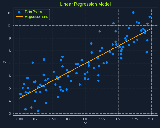
Linear Regression is a fundamental supervised learning algorithm that predicts a continuous target variable by establishing a linear relationship between the target and one or more predictor variables.
The algorithm models this relationship using a linear equation, where changes in the predictor variables result in proportional changes in the target variable. The goal is to find the best-fitting line that minimizes the sum of the squared differences between the predicted values and the actual values.
Imagine you’re trying to predict a house’s price based on size. Linear regression would attempt to find a straight line that best captures the relationship between these two variables. As the size of the house increases, the price generally tends to increase. Linear regression quantifies this relationship, allowing us to predict the price of a house given its size.
What is Regression? #
Before diving into linear regression, it’s essential to understand the broader concept of regression in machine learning.
Regression analysis is a type of supervised learning where the goal is to predict a continuous target variable. This target variable can take on any value within a given range. Think of it as estimating a number instead of classifying something into categories (which is what classification algorithms do).
Examples of regression problems include:
- Predicting the price of a house based on its size, location, and age.
- Forecasting the daily temperature based on historical weather data.
- Estimating the number of website visitors based on marketing spend and time of year.
In all these cases, the output we’re trying to predict is a continuous value. This is what distinguishes regression from classification, where the output is a categorical label (e.g., “spam” or “not spam”).
It’s simply one specific type of regression analysis where we assume a linear relationship between the predictor variables and the target variable. This means we try to model the relationship using a straight line.
Simple Linear Regression #
In its simplest form, simple linear regression involves one predictor variable and one target variable. A linear equation represents the relationship between them:
y = mx + c
yis the predicted target variablexis the predictor variablemis the slope of the line (representing the relationship between x and y)cis the y-intercept (the value of y when x is 0)
The algorithm aims to find the optimal values for m and c that minimize the error between the predicted y values and the actual y values in the training data. This is typically done using Ordinary Least Squares (OLS), which aims to minimize the sum of squared errors.
Multiple Linear Regression #
When multiple predictor variables are involved, it’s called multiple linear regression. The equation becomes:
y = b0 + b1x1 + b2x2 + ... + bnxn
yis the predicted target variablex1,x2, …,xnare the predictor variablesb0is the y-interceptb1,b2, …,bnare the coefficients representing the relationship between each predictor variable and the target variable.
Ordinary Least Squares #

Ordinary Least Squares (OLS) is a common method for estimating the optimal values for the coefficients in linear regression. It aims to minimize the sum of the squared differences between the actual values and the values predicted by the model.
Think of it as finding the line that minimizes the total area of the squares formed between the data points and the line. This “line of best fit” represents the relationship that best describes the data.
Here’s a breakdown of the OLS process:
Calculate Residuals:For each data point, theresidualis the difference between the actualyvalue and theyvalue predicted by the model.Square the Residuals:Each residual is squared to ensure that all values are positive and to give more weight to larger errors.Sum the Squared Residuals:All the squared residuals are summed to get a single value representing the model’s overall error. This sum is called theResidual Sum of Squares(RSS).Minimize the Sum of Squared Residuals:The algorithm adjusts the coefficients to find the values that result in the smallest possible RSS.
This process can be visualized as finding the line that minimizes the total area of the squares formed between the data points and the line.
Assumptions of Linear Regression #
Linear regression relies on several key assumptions about the data:
Linearity:A linear relationship exists between the predictor and target variables.Independence:The observations in the dataset are independent of each other.Homoscedasticity:The variance of the errors is constant across all levels of the predictor variables. This means the spread of the residuals should be roughly the same across the range of predicted values.Normality:The errors are normally distributed. This assumption is important for making valid inferences about the model’s coefficients.
Assessing these assumptions before applying linear regression ensures the model’s validity and reliability. If these assumptions are violated, the model’s predictions may be inaccurate or misleading.
Logistic Regression #

Despite its name, logistic regression is a supervised learning algorithm primarily used for classification, not regression. It predicts a categorical target variable with two possible outcomes (binary classification). These outcomes are typically represented as binary values (e.g., 0 or 1, true or false, yes or no).
For example, logistic regression can predict whether an email is spam or not or whether a customer will click on an ad. The algorithm models the probability of the target variable belonging to a particular class using a logistic function, which maps the input features to a value between 0 and 1.
What is Classification? #
Before we delve deeper into logistic regression, let’s clarify what classification means in machine learning. Classification is a type of supervised learning that aims to assign data points to specific categories or classes. Unlike regression, which predicts a continuous value, classification predicts a discrete label.
Examples of classification problems include:
- Identifying fraudulent transactions (fraudulent or not fraudulent)
- Classifying images of animals (cat, dog, bird, etc.)
- Diagnosing diseases based on patient symptoms (disease present or not present)
In all these cases, the output we’re trying to predict is a category or class label.
How Logistic Regression Works #
Unlike linear regression, which outputs a continuous value, logistic regression outputs a probability score between 0 and 1. This score represents the likelihood of the input belonging to the positive class (typically denoted as ‘1’).
It achieves this by employing a sigmoid function, which maps any input value (a linear combination of features) to a value within the 0 to 1 range. This function introduces non-linearity, allowing the model to capture complex relationships between the features and the probability of the outcome.

The sigmoid function is a mathematical function that takes any input value (ranging from negative to positive infinity) and maps it to an output value between 0 and 1. This makes it particularly useful for modeling probabilities.
The sigmoid function has a characteristic “S” shape, hence its name. It starts with low values for negative inputs, then rapidly increases around zero, and finally plateaus at high values for positive ones. This smooth, gradual transition between 0 and 1 allows it to represent the probability of an event occurring.
In logistic regression, the sigmoid function transforms the linear combination of input features into a probability score. This score represents the likelihood of the input belonging to the positive class.
The Sigmoid Function #
P(x) = 1 / (1 + e^-z)
P(x)is the predicted probability.eis the base of the natural logarithm (approximately 2.718).zis the linear combination of input features and their weights, similar to the linear regression equation:z = m1x1 + m2x2 + ... + mnxn + c
Spam Detection #
Let’s say we’re building a spam filter using logistic regression. The algorithm would analyze various email features, such as the sender’s address, the presence of certain keywords, and the email’s content, to calculate a probability score. The email will be classified as spam if the score exceeds a predefined threshold (e.g., 0.8).
Decision Boundary #

A crucial aspect of logistic regression is the decision boundary. In a simplified scenario with two features, imagine a line separating the data points into two classes. This separator is the decision boundary, determined by the model’s learned parameters and the chosen threshold probability.
In higher dimensions with more features, this separator becomes a hyperplane. The decision boundary defines the cutoff point for classifying an instance into one class or another.
Understanding Hyperplanes #

In the context of machine learning, a hyperplane is a subspace whose dimension is one less than that of the ambient space. It’s a way to visualize a decision boundary in higher dimensions.
- A hyperplane is simply a line in a 2-dimensional space (like a sheet of paper) that divides the space into two regions.
- A hyperplane is a flat plane in a 3-dimensional space (like your room) that divides the space into two halves.
Moving to higher dimensions (with more than three features) makes it difficult to visualize, but the concept remains the same. A hyperplane is a “flat” subspace that divides the higher-dimensional space into two regions.
In logistic regression, the hyperplane is defined by the model’s learned parameters (coefficients) and the chosen threshold probability. It acts as the decision boundary, separating data points into classes based on their predicted probabilities.
Threshold Probability #
The threshold probability is often set at 0.5 but can be adjusted depending on the specific problem and the desired balance between true and false positives.
- If a given data point’s predicted probability
P(x)falls above the threshold, the instance is classified as the positive class. - If
P(x)falls below the threshold, it’s classified as the negative class.
For example, in spam detection, if the model predicts an email has a 0.8 probability of being spam (and the threshold is 0.5), it’s classified as spam. Adjusting the threshold to 0.6 would require a higher probability for the email to be classified as spam.
Data Assumptions #
While not as strict as linear regression, logistic regression does have some underlying assumptions about the data:
Binary Outcome:The target variable must be categorical, with only two possible outcomes.Linearity of Log Odds:It assumes a linear relationship between the predictor variables and the log-odds of the outcome.Log oddsare a transformation of probability, representing the logarithm of the odds ratio (the probability of an event occurring divided by the probability of it not occurring).No or Little Multicollinearity:Ideally, there should be little to nomulticollinearityamong the predictor variables.Multicollinearityoccurs when predictor variables are highly correlated, making it difficult to determine their individual effects on the outcome.Large Sample Size:Logistic regression performs better with larger datasets, allowing for more reliable parameter estimation.
Assessing these assumptions before applying logistic regression helps ensure the model’s accuracy and reliability. Techniques like data exploration, visualization, and statistical tests can be used to evaluate these assumptions.
Decision Trees #

Decision trees are a popular supervised learning algorithm for classification and regression tasks. They are known for their intuitive tree-like structure, which makes them easy to understand and interpret. In essence, a decision tree creates a model that predicts the value of a target variable by learning simple decision rules inferred from the data features.
Imagine you’re trying to decide whether to play tennis based on the weather. A decision tree would break down this decision into a series of simple questions: Is it sunny? Is it windy? Is it humid? Based on the answers to these questions, the tree would lead you to a final decision: play tennis or don’t play tennis.
A decision tree comprises three main components:
Root Node:This represents the starting point of the tree and contains the entire dataset.Internal Nodes:These nodes represent features or attributes of the data. Each internal node branches into two or more child nodes based on different decision rules.Leaf Nodes:These are the terminal nodes of the tree, representing the final outcome or prediction.
Building a Decision Tree #
Building a decision tree involves selecting the best feature to split the data at each node. This selection is based on measures like Gini impurity, entropy, or information gain, which quantify the homogeneity of the subsets resulting from the split. The goal is to create splits that result in increasingly pure subsets, where the data points within each subset belong predominantly to the same class.
Gini Impurity #
Gini impurity measures the probability of misclassifying a randomly chosen element from a set. A lower Gini impurity indicates a more pure set.
Gini(S) = 1 - Σ (pi)^2
Sis the dataset.piis the proportion of elements belonging to classiin the set.
Consider a dataset S with two classes: A and B. Suppose there are 30 instances of class A and 20 instances of class B in the dataset.
- Proportion of class
A:pA = 30 / (30 + 20) = 0.6 - Proportion of class
B:pB = 20 / (30 + 20) = 0.4
The Gini impurity for this dataset is:
Gini(S) = 1 - (0.6^2 + 0.4^2) = 1 - (0.36 + 0.16) = 1 - 0.52 = 0.48
Entropy #
Entropy measures the disorder or uncertainty in a set. A lower entropy indicates a more homogenous set.
Entropy(S) = - Σ pi * log2(pi)
Sis the dataset.piis the proportion of elements belonging to classiin the set.
Using the same dataset S with 30 instances of class A and 20 instances of class B:
- Proportion of class
A:pA = 0.6 - Proportion of class
B:pB = 0.4
The entropy for this dataset is:
Entropy(S) = - (0.6 * log2(0.6) + 0.4 * log2(0.4))
           = - (0.6 * (-0.73697) + 0.4 * (-1.32193))
           = - (-0.442182 - 0.528772)
           = 0.970954
Information Gain #
Information gain measures the reduction in entropy achieved by splitting a set based on a particular feature. The feature with the highest information gain is chosen for the split.
Information Gain(S, A) = Entropy(S) - Σ ((|Sv| / |S|) * Entropy(Sv))
Sis the dataset.Ais the feature used for splitting.Svis the subset ofSfor which featureAhas valuev.
Consider a dataset S with 50 instances and two classes: A and B. Suppose we consider a feature F that can take on two values: 1 and 2. The distribution of the dataset is as follows:
- For
F = 1: 30 instances, 20 classA, 10 classB - For
F = 2: 20 instances, 10 classA, 10 classB
First, calculate the entropy of the entire dataset S:
Entropy(S) = - (30/50 * log2(30/50) + 20/50 * log2(20/50))
           = - (0.6 * log2(0.6) + 0.4 * log2(0.4))
           = - (0.6 * (-0.73697) + 0.4 * (-1.32193))
           = 0.970954
Next, calculate the entropy for each subset Sv:
- For
F = 1:- Proportion of class
A:pA = 20/30 = 0.6667 - Proportion of class
B:pB = 10/30 = 0.3333 - Entropy(S1) =
(0.6667 * log2(0.6667) + 0.3333 * log2(0.3333)) = 0.9183
- Proportion of class
- For
F = 2:- Proportion of class
A:pA = 10/20 = 0.5 - Proportion of class
B:pB = 10/20 = 0.5 - Entropy(S2) =
(0.5 * log2(0.5) + 0.5 * log2(0.5)) = 1.0
- Proportion of class
Now, calculate the weighted average entropy of the subsets:
Weighted Entropy = (|S1| / |S|) * Entropy(S1) + (|S2| / |S|) * Entropy(S2)
                 = (30/50) * 0.9183 + (20/50) * 1.0
                 = 0.55098 + 0.4
                 = 0.95098
Finally, calculate the information gain:
Information Gain(S, F) = Entropy(S) - Weighted Entropy
                       = 0.970954 - 0.95098
                       = 0.019974
Building the Tree #
The tree starts with the root node and selects the feature that best splits the data based on one of these criteria (Gini impurity, entropy, or information gain). This feature becomes the internal node, and branches are created for each possible value or range of values of that feature. The data is then divided into subsets based on these branches. This process continues recursively for each subset until a stopping criterion is met.
The tree stops growing when one of the following conditions is satisfied:
Maximum Depth: The tree reaches a specified maximum depth, preventing it from becoming overly complex and potentially overfitting the data.Minimum Number of Data Points: The number of data points in a node falls below a specified threshold, ensuring that the splits are meaningful and not based on very small subsets.Pure Nodes: All data points in a node belong to the same class, indicating that further splits would not improve the purity of the subsets.
Playing Tennis #

Let’s examine the “Playing Tennis” example more closely to illustrate how a decision tree works in practice.
Imagine you have a dataset of historical weather conditions and whether you played tennis on those days. For example:
| PlayTennis | Outlook_Overcast | Outlook_Rainy | Outlook_Sunny | Temperature_Cool | Temperature_Hot | Temperature_Mild | Humidity_High | Humidity_Normal | Wind_Strong | Wind_Weak |
|---|---|---|---|---|---|---|---|---|---|---|
| No | False | True | False | True | False | False | False | True | False | True |
| Yes | False | False | True | False | True | False | False | True | False | True |
| No | False | True | False | True | False | False | True | False | True | False |
| No | False | True | False | False | True | False | True | False | False | True |
| Yes | False | False | True | False | False | True | False | True | False | True |
| Yes | False | False | True | False | True | False | False | True | False | True |
| No | False | True | False | False | True | False | True | False | True | False |
| Yes | True | False | False | True | False | False | True | False | False | True |
| No | False | True | False | False | True | False | False | True | True | False |
| No | False | True | False | False |
The dataset includes the following features:
Outlook:Sunny, Overcast, RainyTemperature:Hot, Mild, CoolHumidity:High, NormalWind:Weak, Strong
The target variable is Play Tennis: Yes or No.
A decision tree algorithm would analyze this dataset to identify the features that best separate the “Yes” instances from the “No” instances. It would start by calculating each feature’s information gain or Gini impurity to determine which provides the most informative split.
For instance, the algorithm might find that the Outlook feature provides the highest information gain. This means splitting the data based on whether sunny, overcast, or rainy leads to the most significant reduction in entropy or impurity.
The root node of the decision tree would then be the Outlook feature, with three branches: Sunny, Overcast, and Rainy. Based on these branches, the dataset would be divided into three subsets.
Next, the algorithm would analyze each subset to determine the best feature for the next split. For example, in the “Sunny” subset, Humidity might provide the highest information gain. This would lead to another internal node with High and Normal branches.
This process continues recursively until a stopping criterion is met, such as reaching a maximum depth or a minimum number of data points in a node. The final result is a tree-like structure with decision rules at each internal node and predictions (Play Tennis: Yes or No) at the leaf nodes.
Data Assumptions #
One of the advantages of decision trees is that they have minimal assumptions about the data:
No Linearity Assumption:Decision trees can handle linear and non-linear relationships between features and the target variable. This makes them more flexible than algorithms like linear regression, which assume a linear relationship.No Normality Assumption:The data does not need to be normally distributed. This contrasts some statistical methods that require normality for valid inferences.Handles Outliers:Decision trees are relatively robust to outliers. Since they partition the data based on feature values rather than relying on distance-based calculations, outliers are less likely to have a significant impact on the tree structure.
These minimal assumptions contribute to decision trees’ versatility, allowing them to be applied to a wide range of datasets and problems without extensive preprocessing or transformations.
Naive Bayes #

Naive Bayes is a probabilistic algorithm used for classification tasks. It’s based on Bayes' theorem, a fundamental concept in probability theory that describes the probability of an event based on prior knowledge and observed evidence. Naive Bayes is a popular choice for tasks like spam filtering and sentiment analysis due to its simplicity, efficiency, and surprisingly good performance in many real-world scenarios.
Bayes’ Theorem #
Before diving into Naive Bayes, let’s understand its core concept: Bayes' theorem. This theorem provides a way to update our beliefs about an event based on new evidence. It allows us to calculate the probability of an event, given that another event has already occurred.
It’s mathematically represented as:
P(A|B) = [P(B|A) * P(A)] / P(B)
P(A|B): The posterior probability of eventAhappening, given that eventBhas already happened.P(B|A): The likelihood of eventBhappening given that eventAhas already happened.P(A): The prior probability of eventAhappening.P(B): The prior probability of eventBhappening.
Let’s say we want to know the probability of someone having a disease (A) given that they tested positive for it (B). Bayes' theorem allows us to calculate this probability using the prior probability of having the disease (P(A)), the likelihood of testing positive given that the person has the disease (P(B|A)), and the overall probability of testing positive (P(B)).
Suppose we have the following information:
- The prevalence of the disease in the population is 1%, so
P(A) = 0.01. - The test is 95% accurate, meaning if someone has the disease, they will test positive 95% of the time, so
P(B|A) = 0.95. - The test has a false positive rate of 5%, meaning if someone does not have the disease, they will test positive 5% of the time.
- The probability of testing positive,
P(B), can be calculated using the law of total probability.
First, let’s calculate P(B):
P(B) = P(B|A) * P(A) + P(B|¬A) * P(¬A)
P(¬A): The probability of not having the disease, which is1 - P(A) = 0.99.P(B|¬A): The probability of testing positive given that the person does not have the disease, which is the false positive rate,0.05.
Now, substitute the values:
P(B) = (0.95 * 0.01) + (0.05 * 0.99)
     = 0.0095 + 0.0495
     = 0.059
Next, we use Bayes’ theorem to find P(A|B):
P(A|B) = [P(B|A) * P(A)] / P(B)
        = (0.95 * 0.01) / 0.059
        = 0.0095 / 0.059
        ≈ 0.161
So, the probability of someone having the disease, given that they tested positive, is approximately 16.1%.
This example demonstrates how Bayes' theorem can be used to update our beliefs about the likelihood of an event based on new evidence. In this case, even though the test is quite accurate, the low prevalence of the disease means that a positive test result still has a relatively low probability of indicating the actual presence of the disease.
How Naive Bayes Works #
The Naive Bayes classifier leverages Bayes' theorem to predict the probability of a data point belonging to a particular class given its features. To do this, it makes the “naive” assumption of conditional independence among the features. This means it assumes that the presence or absence of one feature doesn’t affect the presence or absence of any other feature, given that we know the class label.
Let’s break down how this works in practice:
Calculate Prior Probabilities:The algorithm first calculates the prior probability of each class. This is the probability of a data point belonging to a particular class before considering its features. For example, in a spam detection scenario, the probability of an email being spam might be 0.2 (20%), while the probability of it being not spam is 0.8 (80%).Calculate Likelihoods:Next, the algorithm calculates the likelihood of observing each feature given each class. This involves determining the probability of seeing a particular feature value given that the data point belongs to a specific class. For instance, what’s the likelihood of seeing the word “free” in an email given that it’s spam? What’s the likelihood of seeing the word “meeting” given that it’s not spam?Apply Bayes' Theorem:For a new data point, the algorithm combines the prior probabilities and likelihoods usingBayes' theoremto calculate theposterior probabilityof the data point belonging to each class. Theposterior probabilityis the updated probability of an event (in this case, the data point belonging to a certain class) after considering new information (the observed features). This represents the revised belief about the class label after considering the observed features.Predict the Class:Finally, the algorithm assigns the data point to the class with the highest posterior probability.
While this assumption of feature independence is often violated in real-world data (words like “free” and “viagra” might indeed co-occur more often in spam), Naive Bayes often performs surprisingly well in practice.
Types of Naive Bayes Classifiers #
The specific implementation of Naive Bayes depends on the type of features and their assumed distribution:
Gaussian Naive Bayes:This is used when the features are continuous and assumed to follow a Gaussian distribution (a bell curve). For example, if predicting whether a customer will purchase a product based on their age and income,Gaussian Naive Bayescould be used, assuming age and income are normally distributed.Multinomial Naive Bayes:This is suitable for discrete features and is often used in text classification. For instance, in spam filtering, the frequency of words like “free” or “money” might be the features, andMultinomial Naive Bayeswould model the probability of these words appearing in spam and non-spam emails.Bernoulli Naive Bayes:This type is employed for binary features, where the feature is either present or absent. In document classification, a feature could be whether a specific word is present in the document.Bernoulli Naive Bayeswould model the probability of this presence or absence for each class.
The choice of which type of Naive Bayes to use depends on the nature of the data and the specific problem being addressed.
Data Assumptions #
While Naive Bayes is relatively robust, it’s helpful to be aware of some data assumptions:
Feature Independence:As discussed, the core assumption is that features are conditionally independent given the class.Data Distribution:The choice of Naive Bayes classifier (Gaussian, Multinomial, Bernoulli) depends on the assumed distribution of the features.Sufficient Training Data:Although Naive Bayes can work with limited data, it is important to have sufficient data to estimate probabilities accurately.
Support Vector Machines (SVMs) #

Support Vector Machines (SVMs) are powerful supervised learning algorithms for classification and regression tasks. They are particularly effective in handling high-dimensional data and complex non-linear relationships between features and the target variable. SVMs aim to find the optimal hyperplane that maximally separates different classes or fits the data for regression.
Maximizing the Margin #
An SVM aims to find the hyperplane that maximizes the margin. The margin is the distance between the hyperplane and the nearest data points of each class. These nearest data points are called support vectors and are crucial in defining the hyperplane and the margin.
By maximizing the margin, SVMs aim to find a robust decision boundary that generalizes well to new, unseen data. A larger margin provides more separation between the classes, reducing the risk of misclassification.
Linear SVM #
A linear SVM is used when the data is linearly separable, meaning a straight line or hyperplane can perfectly separate the classes. The goal is to find the optimal hyperplane that maximizes the margin while correctly classifying all the training data points.
Finding the Optimal Hyperplane #
Imagine you’re tasked with classifying emails as spam or not spam based on the frequency of the words “free” and “money.” If we plot each email on a graph where the x-axis represents the frequency of “free” and the y-axis represents the frequency of “money,” we can visualize how SVMs work.

The optimal hyperplane is the one that maximizes the margin between the closest data points of different classes. This margin is called the separating hyperplane. The data points closest to the hyperplane are called support vectors, as they “support” or define the hyperplane and the margin.
Maximizing the margin is intended to create a robust classifier. A larger margin allows the SVM to tolerate some noise or variability in the data without misclassifying points. It also improves the model’s generalization ability, making it more likely to perform well on unseen data.
In the spam classification scenario depicted in the graph, the linear SVM identifies the line that maximizes the distance between the nearest spam and non-spam emails. This line serves as the decision boundary for classifying new emails. Emails falling on one side of the line are classified as spam, while those on the other side are classified as not spam.
The hyperplane is defined by an equation of the form:
w * x + b = 0
wis the weight vector, perpendicular to the hyperplane.xis the input feature vector.bis the bias term, which shifts the hyperplane relative to the origin.
The SVM algorithm learns the optimal values for w and b during the training process.
Non-Linear SVM #

In many real-world scenarios, data is not linearly separable. This means we cannot draw a straight line or hyperplane to perfectly separate the different classes. In these cases, non-linear SVMs come to the rescue.
Kernel Trick #
Non-linear SVMs utilize a technique called the kernel trick. This involves using a kernel function to map the original data points into a higher-dimensional space where they become linearly separable.
Imagine separating a mixture of red and blue marbles on a table. If the marbles are mixed in a complex pattern, you might be unable to draw a straight line to separate them. However, if you could lift some marbles off the table (into a higher dimension), you might be able to find a plane that separates them.
This is essentially what a kernel function does. It transforms the data into a higher-dimensional space where a linear hyperplane can be found. This hyperplane corresponds to a non-linear decision boundary when mapped back to the original space.
Kernel Functions #
Several kernel functions are commonly used in non-linear SVMs:
Polynomial Kernel:This kernel introduces polynomial terms (like x², x³, etc.) to capture non-linear relationships between features. It’s like adding curves to the decision boundary.Radial Basis Function (RBF) Kernel:This kernel uses a Gaussian function to map data points to a higher-dimensional space. It’s one of the most popular and versatile kernel functions, capable of capturing complex non-linear patterns.Sigmoid Kernel:This kernel is similar to the sigmoid function used in logistic regression. It introduces non-linearity by mapping the data points to a space with a sigmoid-shaped decision boundary.
The kernel function choice depends on the data’s nature and the model’s desired complexity.
Image Classification #
Non-linear SVMs are particularly useful in applications like image classification. Images often have complex patterns that linear boundaries cannot separate.
For instance, imagine classifying images of cats and dogs. The features might be things like fur texture, ear shape, and facial features. These features often have non-linear relationships. A non-linear SVM with an appropriate kernel function can capture these relationships and effectively separate cat images from dog images.
The SVM Function #
Finding this optimal hyperplane involves solving an optimization problem. The problem can be formulated as:
Minimize: 1/2 ||w||^2
Subject to: yi(w * xi + b) >= 1 for all i
wis the weight vector that defines the hyperplanexiis the feature vector for data pointiyiis the class label for data pointi(-1 or 1)bis the bias term
This formulation aims to minimize the magnitude of the weight vector (which maximizes the margin) while ensuring that all data points are correctly classified with a margin of at least 1.
Data Assumptions #
SVMs have few assumptions about the data:
No Distributional Assumptions:SVMs do not make strong assumptions about the underlying distribution of the data.Handles High Dimensionality:They are effective in high-dimensional spaces, where the number of features is larger than the number of data points.Robust to Outliers:SVMs are relatively robust to outliers, focusing on maximizing the margin rather than fitting all data points perfectly.
SVMs are powerful and versatile algorithms that have proven effective in various machine-learning tasks. Their ability to handle high-dimensional data and complex non-linear relationships makes them a valuable tool for solving challenging classification and regression problems.